An **extremum** (or extreme value) of a function is a point at which a **maximum** or **minimum** value of the function is obtained in some interval.
Consider Figure 3.1.1:
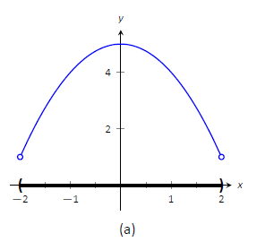
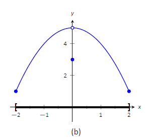
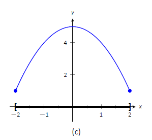
If \(f\) is continuous on a closed interval \([a, b]\), then \(f\) attains an absolute maximum value stem:[f(c)] and an absolute minimum value \(f(d)\) at some numbers \(c\) and \(d\) in \([a, b]\).
Functions continuous on a closed interval always attain extreme values.
If \(f\) has a local maximum or minimum at \(c\), and if \(f^\prime(c)\) exists, then \(f^\prime(c) = 0\).
In terms of critical numbers, Fermat’s Theorem can be rephrased as follows:
If f has a local maximum or minimum at c, then c is a critical number of f.
Critical numbers include when \(f^\prime(x) = \text{undefined}\), but, \(f(c)\) must be defined.
For example, consider the following function:
While \(f^\prime(x)\) is undefined at \(x = 3\), \(f(3)\) is likewise undefined, therefore, \(x = 3\) is not a critical number.
TODO: double check this...
Also points where \(f(x) = \text{undefined}\) and where \(f^\prime(x) = \text{undefined}\) is still useful for calculating other details such as intervals of increase or decrease.
A critical number of a function \(f\) is a number \(c\) in the domain of \(f\) such that either
To find an absolute maximum or minimum of a continuous function on a closed interval, we note that either it is local [in which case it occurs at a critical number by (7)] or it occurs at an endpoint of the interval, as we see from the examples in Figure 8. Thus the following three-step procedure always works. **See The Closed Interval Method.**
To find the absolute maximum and minimum values of a continuous function \(f\) on a closed interval \([a, b]\):
I.e. the maximum/minimum of \(f^\prime(c) = 0\), \(f(a)\), and \(f(b)\).
Using sudo code, the 'The Closed Interval Method' can be defined as the result of:
In mathematics, the mean value theorem states, roughly, that for a given planar arc between two endpoints, there is at least one point at which the tangent to the arc is parallel to the secant through its endpoints.
For any function that is continuous \([a, b]\) and differentiable on \((a,b)\), there exists some \(c\) in the interval \((a,b)\) such that the secant joining the endpoints of the \([a, b]\) is parallel to the tangent at \(c\):

The function f attains the slope of the secant between a and b as the derivative at the point \({\displaystyle \xi \in (a,b)}\):

It is also possible that there are multiple tangents parallel to the secant:

We will see that many of the results of this chapter depend on one central fact, which is called the Mean Value Theorem. But to arrive at the Mean Value Theorem we first need the following result.
Let f be a function that satisfies the following three hypotheses:
Then there is a number \(c\) in \((a, b)\), such that \(f^\prime(c) = 0\)
Let \(f\) be a function that satisfies the following hypotheses:
Then there is a number \(c\) in \((a, b)\), such that: \(\begin{equation} \begin{split} f^\prime(c) &= \frac{f(b) - f(a)}{b - a} \end{split} \end{equation}\) Or, equivalently: \(\begin{equation} \begin{split} f(b) - f(a) &= f^\prime(c)(b - a) \end{split} \end{equation}\) Where the tangent at \(c\) is parallel to the secant line through the endpoints \((a, f(a))\) and stem:[(b, f(b))].
The Mean Value Theorem is an example of what is called an existence theorem. Like the Intermediate Value Theorem, the Extreme Value Theorem, and Rolle’s Theorem, it guarantees that there exists a number with a certain property, but it doesn’t tell us how to find the number.
If stem:[f^\prime(x) = 0] for all x in an interval \((a, b)\), then f is constant on \((a, b)\).
if stem:[f^\prime(x) = g^\prime(x)] for all stem:[x] in an interval \((a, b)\), then stem:[f - g] is constant on \((a, b)\); that is, stem:[f(x) = g(x) + c] where \(c\) is a constant.
Corollary 7 says that if two functions have the same derivatives on an interval, then their graphs must be vertical translations of each other there. In other words, the graphs have the same shape, but could be shifted up or down.
Many of the applications of calculus depend on our ability to deduce facts about a function f from information concerning its derivatives.
Because stem:[f^\prime(x)] represents the slope of the curve stem:[y = f(x)] at the point stem:[(x, f(x))], it tells us the direction in which the curve proceeds at each point. So it is reasonable to expect that information about stem:[f^\prime(x)] will provide us with information about stem:[f(x)].
If \(f^\prime(x) > 0\) on an interval, then \(f(x)\) is increasing on that interval.
I.e. the tangent lines (in the \(f(x)\) interval) have positive slope.If \(f^\prime(x) < 0\) on an interval, then \(f(x)\) is decreasing on that interval.
I.e. the tangent lines (in the \(f(x)\) interval) have negative slope.Suppose that c is a critical number of a continuous function f:
[†]: 'at \(c\)' means from the left and right of the given point.
If the graph of f lies above all of its tangents on an interval I, then it is called concave upward on I. If the graph of f lies below all of its tangents on I, it is called concave downward on I.
For a function \(f(x)\) with derivatives \(f^\prime\) and \(f^{\prime\prime}\) on an interval the following holds:
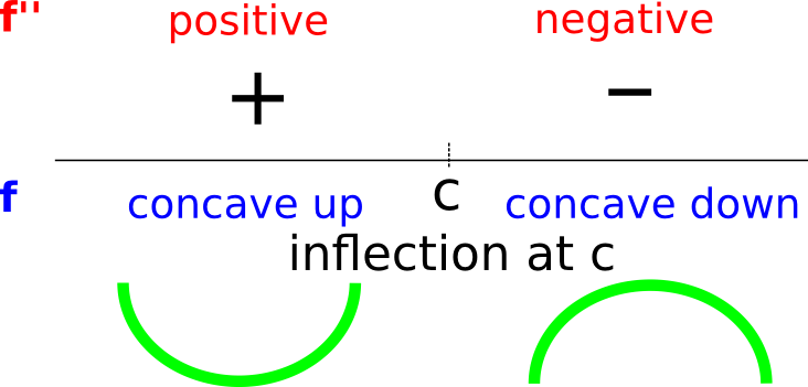
This means that the function is concave down before \(c\), concave up after \(c\) and has an inflection point at \(x = c\).
For Example:
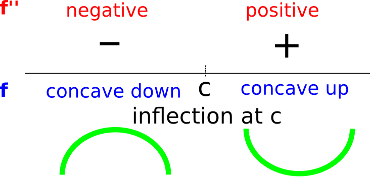
This means that the function is concave up before \(c\), concave down after \(c\), and has an inflection point at \(x = c\).
For Example:
(I.e. it is either positive both before or after \(c\) or negative both before or after \(c\))
In this case, f does not have an inflection point at \(x = c\).
For Example:
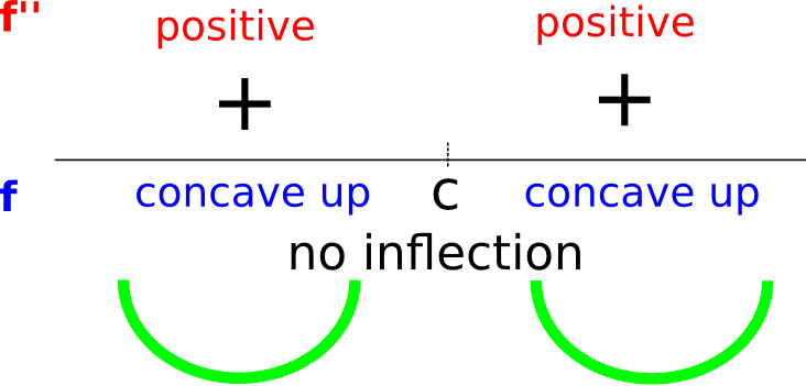
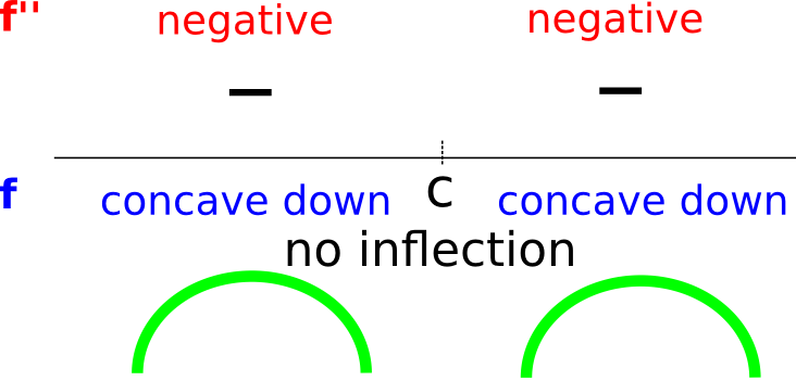
The existence of the third case demonstrates that a function does not necessarily have an inflection point at a critical point of \(f^\prime\).
Using the number line test for \(f^{\prime\prime}\) one can both determine the intervals on which \(f\) is concave up/down as well as classify the critical point of \(f^{\prime}\) into three categories matching the three cases above and determine the inflection points.
To determine the inflection points a differentiable function \(f(x)\)
Concavity of the function can also be used to determine if there is an extreme value or not at a critical point of \(f\).
Remember:
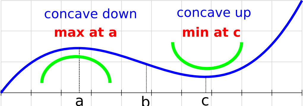
Thus, if \(c\) is a critical point and the second derivative at \(c\) is positive, that means that the function is concave up around \(c\). Thus, there is a relative minimum at \(c\).
Conversely, if \(c\) is a critical point and the second derivative at \(c\) is negative, that means that the function is concave down around \(c\). Thus, there is a relative maximum at \(c\).
If \(f^{\prime\prime} = 0\) this test is inconclusive (i.e. probably an inflection point).
This procedure of determining the extreme values is known as the Second Derivative Test.
When the second derivative is zero, it corresponds to a possible inflection point.
A point stem:[P] on a curve stem:[y = f(x)] is called an inflection point if \(f\) is continuous there and the curve changes from concave upward to concave downward or from concave downward to concave upward at stem:[P].
If \(f(x)\) has an inflection point at \(x = c\), then \(f^{\prime\prime}(c) = 0\) or \(f^{\prime\prime}(c)\) does not exist.
Example: Determine the intervals on which the function with the graph on the right defined on interval (a, ∞) is concave up/down.
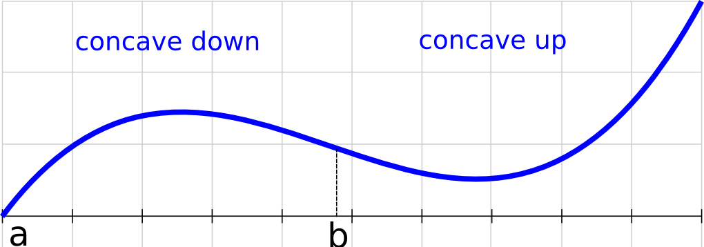
Solution: The function is concave up on the interval (a,b) and concave down on the interval (b, ∞).
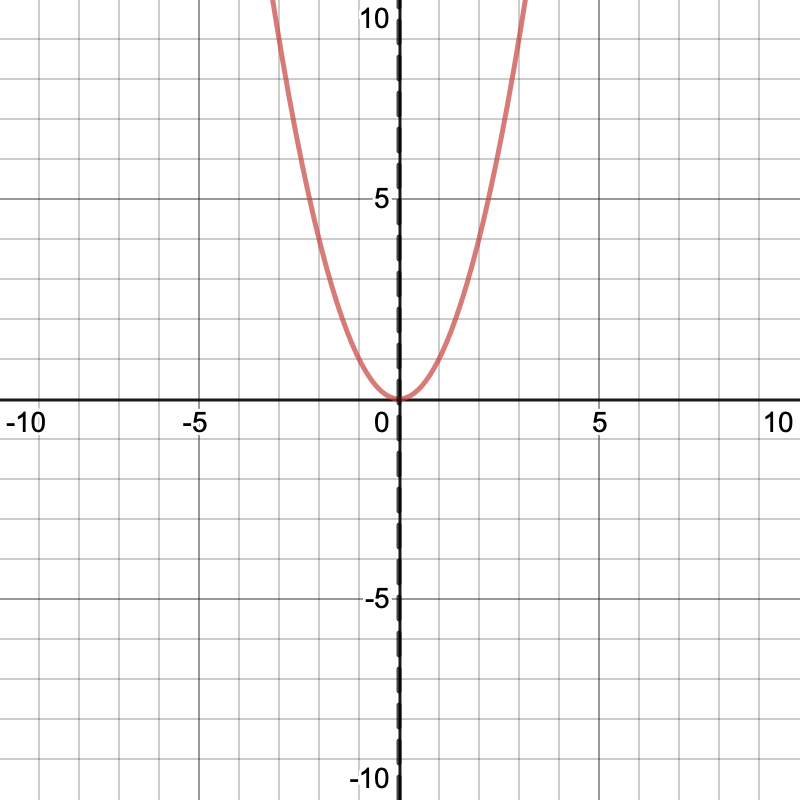
Quadratic functions have no points of inflection:
Suppose \(f^{\prime\prime}\) is continuous near c:
The Second Derivative Test is inconclusive when stem:[f^{\prime\prime}(c) = 0]. In other words, at such a point there might be a maximum, there might be a minimum, or there might be neither (as in Example 6). This test also fails when stem:[f^{\prime\prime}(c)] does not exist. In such cases the First Derivative Test must be used. In fact, even when both tests apply, the First Derivative Test is often the easier one to use.
The second derivative may be used to determine local extrema of a function under certain conditions. If a function has a critical point for which \(f^\prime(x) = 0\) and the second derivative is positive at this point, then \(f\) has a local minimum here.
Which makes sense, because \(-\infty \not\equiv \infty\). Since, in the case of horizontal asymptotes:
Or rather is unbounded in the given direction.
**The professor said:** you can't just apply the limit laws, such as for:
Because we don't know if it is continuous.
\(\)
For e.g. horizontal asymptotes, don't forgot to add \(y = x\), don't just say \(x\)
Check that there is no division with 0, or even roots of negative numbers.
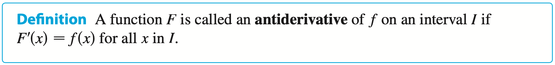
If \(f(-x) = f(x)\) then \(f\) is even and will be symmetric about the y-axis.
If \(f(x) = f(x + p)\) where \(p\) is a positive constant, then \(f\) is a periodic function, and it's graph will be repeated every \(p\) units (i.e. the period).
\(p\) is the period I believe, such as \(\pi\)
Asymptotes of e.g. rational functions can be found using the first and second derivatives, instead of using vertical and horizontal limits.
Steps:
See §1.5 | The Limit of a Function.
Usually (but not always) this will involve checking to see where the denominator equals zero.
The vertical asymptotes occur only when the denominator is zero (If both the numerator and denominator are zero, the multiplicities of the zero are compared).
For example, the following function has vertical asymptotes at \(x = 0\), and \(x = 1\), but not at \(x = 2\).
See 3.4 | Limits at Infinity; Horizontal Asymptotes.
A slant (oblique) asymptote occurs when the polynomial in the numerator is a higher degree than the polynomial in the denominator.
Can be found using polynomial long division, where the quotient \(mx + b\) is your slant asymptotes, then set \(y = mx + b\).
The above result can be confirmed using limits. Given some \(y = mx + b\), if:
Find the intervals where:
Use the I/D Test.
Find the intervals where:
Check for points of inflection(points where \(f^{\prime\prime}\) changes sign).
In some cases you can also use Second Derivative Test to test for local maximum and minimum values.
Sketch asymptotes as dashed lines. Plot intercepts, critical points, and inflection points. Draw a curve through these points which is consistent with the information found in the previous parts.
For instance, given \(y = x^3\), the number line for the first and second derivatives will look like:

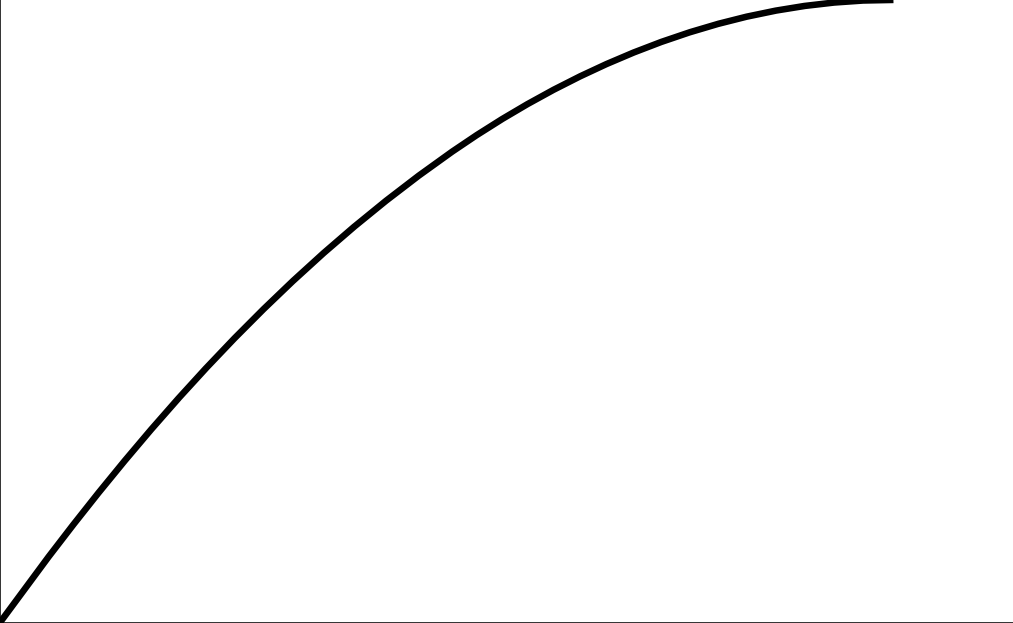
On the negative (left) side, since \(f^\prime\) is positive, and \(f^{\prime\prime}\) is negative, it is increasing at a decreasing rate. So the curve will look like this
Whereas on the positive (right) side of x, since the first derivative is positive and the second derivative is likewise positive, it will be increasing at an increasing rate. So therefore, the curve will look like this:
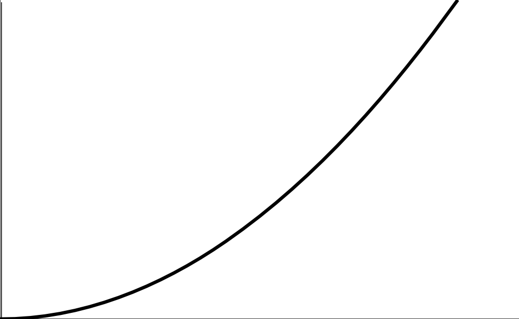
Which matches the (compressed) curve of:
This process works for asymptotes as well, such as those from rational functions.
Well we know that the derivative of \(x^2\) is \(2x\), so therefore:
So therefore, the above graph is not a function of \(x^2\).
This graph satisfies the aforementioned constraints of:
But for the same reasons, it is not a function of \(x^2\).
Given two additional points left of \(a\), and right of \(a\)
It's easier to use \(f^{\prime\prime}(a)\) instead.
Use the first derivative to find increasing & decreasing intervals (by testing the left and right sides of \(f^\prime(a)\)).
The first derivative can yield concavity information (by testing the left and right points of \(f^\prime(a)\)), but only for extrema points.
Can also use the The Closed Interval Method
Suppose that \(c\) is a critical number of a continuous function \(f\) defined on an interval.
If:
Then \(f(x)\) is the absolute maximum value of \(f\).
If:
Then \(f(x)\) is the absolute minimum value of \(f\).
An alternative method for solving optimization problems is to use implicit differentiation.
Remember: